The Invisible Wall Around Hash Tables
Why we believed reordering was essential — and what happens when someone proves it’s not
We’ve all done it.
You’re building a hash table. Open addressing. Greedy insertion. Straightforward: hash the key, scan forward until you find an empty slot, drop it in.
And yeah, we know the performance hit $ \Theta(\log(1/\delta)) $ probes as the table fills up. That’s what Yao proved in the 80s. Ullman saw it coming even earlier. We’ve lived with that bound as if it’s gravity.
What does \(\Theta(\log(1/\delta))\) actually mean?
This bit of notation might look like a maths flex, but it describes something clear:
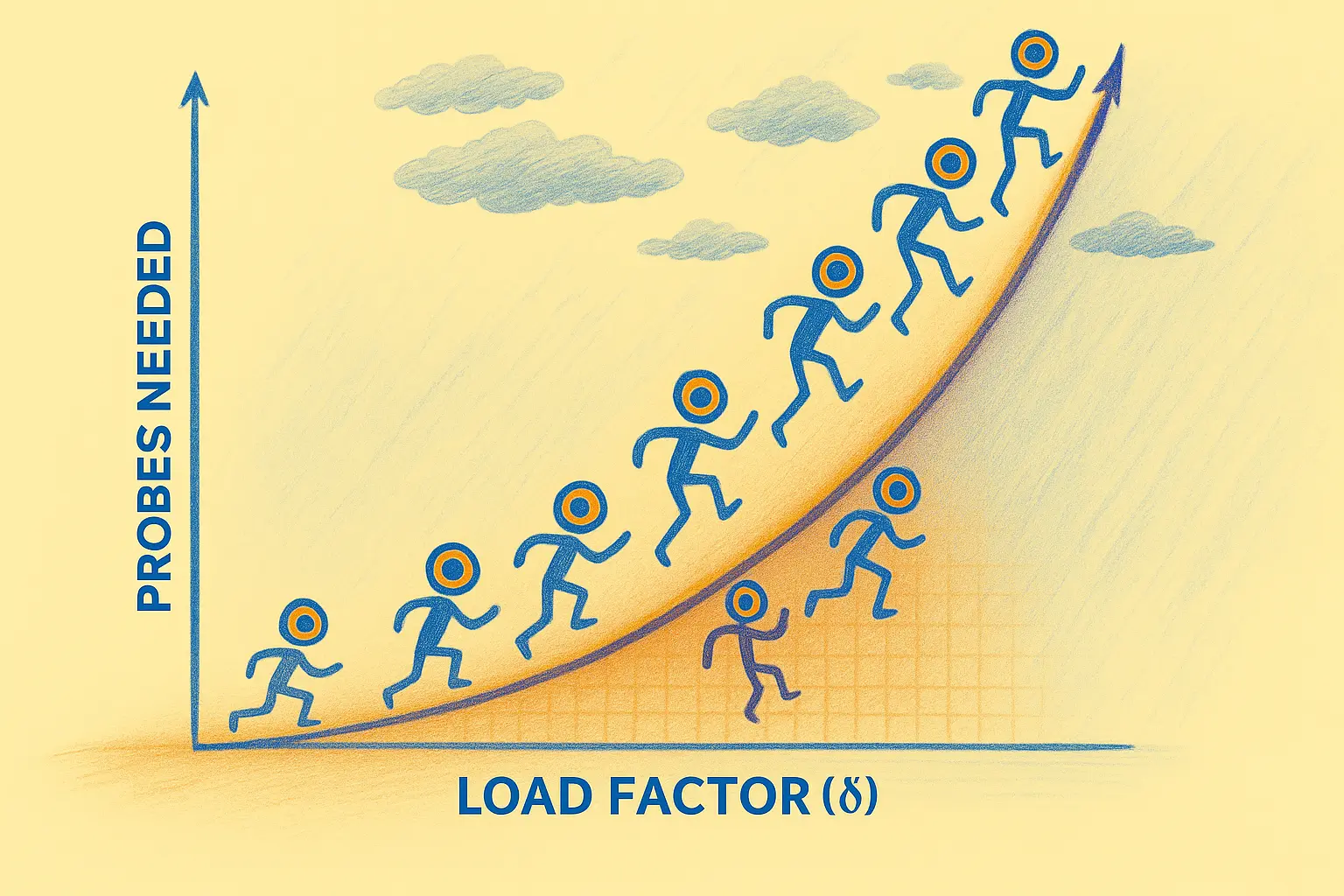
- $ \delta $ is how full your hash table is. If it’s 90% full, then $ \delta = 0.9 $.
- \(1/\delta\) tells you how little room is left. \(1/0.9 \approx 1.11\) — not much room left.
- Taking the log? That grows slowly at first, but steeply as ( \delta \to 1 ).
Here’s what it feels like:
| Load Factor | Log Term | Probes Needed |
|---|---|---|
| 0.5 | 0.30 | few |
| 0.75 | 0.58 | more |
| 0.9 | 1.00 | lots |
| 0.99 | 2.00 | painful |
| 0.999 | 3.00 | why |
Takeaway:
Even though \( \log(1/\delta)\) grows slowly, the tail end hurts.
Greedy insertions struggle badly once tables get nearly full.
That “law”? Not really a law. Just a habit.
The mental model we never questioned
The story was: if you don’t reorder elements, you can’t beat \(\Theta(\log(1/\delta))\) probe complexity. Most improvements tried to sidestep the rule — move keys around after insertions, or use clever backup schemes.
Recent research reveals something big: you can break that bound — without any clever reordering. No reordering. No cleanup. Just stop being greedy.
Let’s see what that actually means.
What’s the state of the art?
Most modern hash tables don’t just do naive linear probing. We’ve gotten smarter — but not that much smarter.
Here’s what’s common today:
- Linear Probing: Fast and cache-friendly, but clusters badly under load.
- Quadratic Probing: Spreads out collisions better but can still form secondary clusters.
- Double Hashing: Uses a second hash to avoid predictable probe sequences. Good in theory, finicky in practice.
- Robin Hood Hashing: Tries to balance probe lengths by stealing slots from rich (short-probe) keys. It helps — but requires reordering.
- Hopscotch and Cuckoo Hashing: Push even further to avoid clusters. Both reorder aggressively and juggle entries to keep probe lengths low.
Each of these try to dodge the log-bound in their own way — but they either:
- reorder entries, or
- introduce more bookkeeping (like tracking probe lengths or relocation windows).
Which makes sense, right? If you assume greedy is your only move, your only fix is to clean up afterwards.
What if you didn’t need to?
Seeing Greedy in Action
We’ll start with the classic greedy insert, and add a simple visualisation so you can see the clustering happen.
Here’s the core logic:
pub fn insert_greedy(&mut self, key: K, value: V) -> usize {
    let mut probes = 0;
    loop {
        let idx = (self.hash(&key) + probes) % self.table.len();
        if self.table[idx].is_none() {
            self.table[idx] = Some((key, value));
            return probes + 1;
        }
        probes += 1;
    }
}
Each key just walks forward until it finds a spot. Direct. Deadly.
Run it yourself
If you want to feel the slowdown, here’s a Rust demo you can tweak live:
https://github.com/oliverdaff/hash-tables-without-assumptions
cargo run --bin post1-invisible-wall
Or customise it:
cargo run --bin post1-invisible-wall -- --slots 40 --keys 25
You can also control the hashing behaviour:
# Use real-world hashing (DefaultHasher) — the default
cargo run --bin post1-invisible-wall -- --slots 40 --keys 25

# Force terrible clustering with a mod-10 hash
cargo run --bin post1-invisible-wall -- --slots 40 --keys 25 --hash-strategy mod10
A note about hashing
By default, we use Rust’s DefaultHasher — the same randomised SipHash that production systems use.
No tricks. No cheating. Keys land evenly unless you’re deliberately chasing chaos.
If you want to see worst-case clustering — to feel the wall hit even harder — you can switch to a deliberately bad hash (mod10).
HashTable Config Example
When you run it, you’ll see something like:
cargo run --bin post1-invisible-wall
HashTable Config:
  - Slots: 30
  - Keys: 0..14
  - Hash strategy: Default

Hash Table View:

  [ ]  [2]  [4]  [9]  [ ] [11]  [ ]  [5]  [ ]  [ ]
  [7]  [ ]  [ ]  [ ]  [ ] [12]  [ ]  [8]  [ ] [13]
  [0] [14]  [3] [10]  [1]  [ ]  [ ]  [ ]  [ ]  [6]
or if you force a bad hash:
cargo run --bin post1-invisible-wall -- --hash-strategy=mod10

HashTable Config:
  - Slots: 30
  - Keys: 0..14
  - Hash strategy: Mod10

Hash Table View:

  [0]  [1]  [2]  [3]  [4]  [5]  [6]  [7]  [8]  [9]
 [10] [11] [12] [13] [14]  [ ]  [ ]  [ ]  [ ]  [ ]
  [ ]  [ ]  [ ]  [ ]  [ ]  [ ]  [ ]  [ ]  [ ]  [ ]
It’s all explicit — no surprises.
Measuring the Invisible Wall
Demos are fun, but we also measured it properly.
We benchmarked insertion times at across different load factors —
then plotted them.
Here’s what happens:
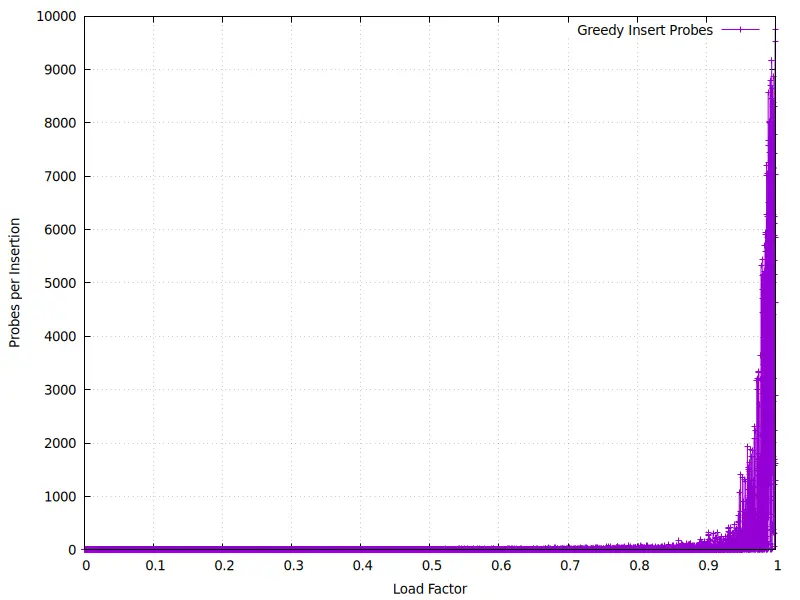
Take a look at the right end.
Greedy looks fine… until about 90% full.
After that, things quickly unravel.
How we did it
We took two different measurements:
Measuring probes per insertion
We wanted to see the real invisible wall — how the number of probes needed grows as the table fills up.
Commands:
just probes_at_load
just plot_probe_time
The first command inserts keys one-by-one into a large table,
recording the load factor and the number of probes used for each insertion.
The second plots probes per insertion against load factor.
This highlights the raw logarithmic slowdown without any averaging effects.
Measuring average insertion time
We also measured the practical impact — how slow greedy insertion feels when inserting many keys at once.
Commands:
just bench
just bench-report
The bench command runs Criterion benchmarks at five load factors (50%, 75%, 90%, 95%, 99%), then bench-report opens the bench mark graphs in your browser.
This shows how quickly performance degrades under real-world usage as the tables fill up.
Two measurements, two graphs, two ways to see the invisible wall.
Explore the Code
You can grab the repo:
git clone https://github.com/oliverdaff/hash-tables-without-assumptions
cd hash-tables-without-assumptions
Then:
just post1
just bench
just bench-report
or with nix
nix develop -c just post1
nix develop -c just bench
nix develop -c just bench-report
We use just for shortcuts, flake.nix for reproducibility
Next up:
How to break the wall — without reordering anything.
Elastic insertions, sub-logarithmic probes, and fairer hashing.
It gets better.